Intro
to Probability and Statistics
Sample
Final #3 – Questions And Answers (Answer Key)
Professor Brian Shydlo
Instructions:
1) Please
write your name: _____________________________________
2) There
are 7 questions totaling 100 points. Please be careful to answer all questions.
Partial credit will be given.
Question 1)
16 Points
Question 2)
18 Points
Question
3) 6 Points
Question 4)
15 Points
Question 5)
18 Points
Question 6)
21 Points
Question
7) 6 Points
Total:
100 Points
Question
1) (15 points in total)
A certain
stock, X, has an expected return of 20%
per year and a standard deviation of 25%.
A certain
bond, Y, has an expected return of 5%
per year and a standard deviation of 9%.
The have a
correlation of -0.2.
You could
write this as:
mx
= 20, my
= 5, sx
= 25, sy
= 9, and rxy = -0.2.
Question
1a) (3 Points)
You decide
to invest $100 dollars in either X or Y or some combination of both. How do you allocate your $100 to maximize
your expected return?
Answer 1a) Invest all $100 in X.
Question
1b) (3 Points)
You
remember hearing something about diversification in an investments class. So you decide to split your money and invest
$50 in X and $50 in Y. How much money do
you expect to have after one year (your initial investment of $100 + the
expected return of your portfolio of X and Y).
Answer 1b)
$100
* [ 50% * 20% + 50% * 5%] =
$100
* [ 10% + 2.5%] =
$100
* [ 12.5%] =
$112.50
Question
1c) (6 Points)
What is the
standard deviation and variance of the portfolio from part b?
Answer 1c)
Variance(whole portfolio) = (Psx)2 + ((1-P)sy)2 + 2 * (Psx) * ((1-P)sy)) * rxy
Variance(whole portfolio) = (.5 * 25)2
+ (.5 * 9)2 + 2 * (.5 * 25) *
(.5 * 9)) * -0.2
Variance(whole portfolio) = (12.5)2 +
(4.5)2 + 2 * (12.5) * (4.5) *
-0.2
Variance(whole portfolio) = 156.25 + 20.25 + -22.5
Variance(whole portfolio) = 154
Standard Deviation of Whole Portfolio = sqrt(154) = 12.41
Question
1d) (4 Points)
What is a
95% (2 standard deviation) confidence interval for your return? That is, give me a confidence interval for
50% in X and 50% in Y.
Answer 1d)
P[12.5
- (2 * 12.41) < μ < 12.5 + (2 * 12.41)] = 95%
P[12.5
- 24.82 < μ < 12.5 + 24.82] = 95%
P[-12.32
< μ < 37.32] = 95%
Question
2) (18 Points in total)
A city
decides to determine the mean expenditures per tourist per visit. A random sample of 100 finds that the average
expenditure is $800. The standard
deviation of expenditures for all tourists is $120.
Question
2a) (6 Points)
What is the
standard deviation of the mean, given that the standard deviation of the whole
population is $120 and the number of people sampled is 100?
Answer 2a)
s x = 120
s x-bar = 120 / Sqrt(100) =
120 / 10 = 12
s x-bar = 12
Question
2b) (6 Points)
What is a
95% (2 standard deviation) confidence interval for the value of the
expenditures per tourist?
Answer 2b)
P[800
- (2*12)
< μ < 800 + (2*12) ]
= 95%
P[800
- 24 <
μ < 800
+ 24] = 95%
P[776 < μ < 824] = 95%
Question
2c) (6 Points)
If the city
wants the error of estimation to be $20, how many people does it need to
sample? (If this helps, remember that
the error of estimation is equal to half the width of the confidence interval.)
Answer 2c)
n =
(22 x 1202) / 202 = 144
They
would have to sample 144 people.
Question
3) (6 points in total)
On the
following graph, one of the lines is the Z distribution and the other is the T
Distribution with 2 degrees of freedom.
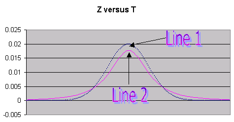
Question
3a) (6 Points)
Is Line 1
the Z distribution or the T distribution with 2 degrees of freedom?
Answer 3a)
Line
1 is the Z Distribution.
Line
2 is the T Distribution with 2 degrees of freedom.
Question
4) (15 Points)
The average
distance of stopping a certain make of automobile is 65 feet. A company deigns a new brake thought to be
more effective than the type they currently use. To test this brake, they install it on 64
cars. The new brakes give a stopping
distance of 63 feet with a standard deviation of 4 feet.
Question
4a) (5 Points)
Formulate a
hypothesis for a lower-tail test. (i.e.
write the null hypothesis and the alternate hypothesis).
Answer 4a)
H0: μ = 65 or μ >= 65
H1: μ < 65 or Ha: μ < 65
Line
1 is the Z Distribution.
Line
2 is the T Distribution with 2 degrees of freedom.
Question
4b) (5 Points)
Construct
the Z statistic to test how many standard deviations is the sample mean of 63
away from the original mean of 65.
Answer 4b)
s x-bar = 4 / Sqrt(64) =
0.5
Z
= (63 - 65) / 0.5 = -4.00
Question
4c) (5 Points)
Are the new
brakes significantly better than the old brakes? Significant is this case means 95%.
Answer 4c)
Yes,
the new brakes are significantly better.
-4 is well to the left of the -1.65 threshold required for a lower-tail
test.
Question
5) (18 points) Someone
starts a new mutual fund that invests based on the winner of the Superbowl.
Quoted from
a newspaper from January 2001:
"One of the quirkiest stock market indicators is the so called Super Bowl predictor for the market. If the Super Bowl is won by a team from the original, pre-merger National Football League, the market will close higher by the end of the year. If a team from the old American Football League wins, then the market will fall."
Here is
data from the market over the last 10 years:
|
# |
Year |
Stock Market Return |
Old NFL Wins (Yes/No) |
Old NFL Wins (1/0) |
Prediction Correct |
|
1 |
1991 |
30 |
Yes |
1 |
Yes |
|
2 |
1992 |
-2 |
Yes |
1 |
No |
|
3 |
1993 |
20 |
Yes |
1 |
Yes |
|
4 |
1994 |
-2 |
No |
0 |
Yes |
|
5 |
1995 |
50 |
Yes |
1 |
Yes |
|
6 |
1996 |
40 |
Yes |
1 |
Yes |
|
7 |
1997 |
-20 |
Yes |
1 |
No |
|
8 |
1998 |
40 |
Yes |
1 |
Yes |
|
9 |
1999 |
60 |
Yes |
1 |
Yes |
|
10 |
2000 |
-5 |
No |
0 |
Yes |
If the old
NFL (National Football League)) wins the mutual fund puts their money into the
stock market, that is, they bet it will go up.
Otherwise if they bet it will go down.
If you look at the table above, you'll see that the prediction was
correct 8 out of 10 times or 80% of the time.
It was only wrong in 1992 and 1997.
You decide
to test out this theory by doing a simple linear regression. For the X (predictor variable) you use Old
NFL Wins (0 for no and 1 for yes). For the Y you use Stock Market Return. You run this through Minitab and this is the
output you get.
The regression equation is
Stock Return = - 3.5 + 30.7
Old NFL Wins?
Predictor Coef StDev T P
Constant -3.50 17.80 -0.20
0.849
NFL Wins 30.75 19.90 1.55
0.161
S = 25.17 R-Sq =
23.0% R-Sq(adj) = 13.4%
Analysis of Variance
Source DF
SS MS F P
Regression 1
1512.9 1512.9 2.39
0.161
Residual Error 8
5068.0 633.5
Total 9 6580.9
Question
5a) (6 Points)
Based on the Minitab output, comment and interpret on whether or not it the
regression model is valid in this case.
Answer 5a) The P score is too high. We typically want something below
0.05. This is above 0.05, in fact, it is
0.161. This suggests that random
fluctuations could have caused the stock market movements and not necessarily
the Superbowl.
Of
course, as we know, correlation does not imply causality.
Question
5b) (6 Points) This year, the Baltimore Ravens won, and they
are not part of the old NFL (they were part of the AFL), so the rule says that
the stock market should go down.
What is
your prediction of the return on the stock market based on the regression
equation from Minitab from part a?
(Regardless
of whether or not the regression is valid, I still want your prediction.)
Answer 5b) The regression equation is:
Stock Return = -3.5 + ( 30.7 * NFL Wins? )
So
in this case, NFL Wins is 0. Plug into
the formula:
Predicted
Stock Return = -3.5 + ( 30.7 * 0 )
Predicted
Stock Return = -3.5 + 0
Predicted
Stock Return = -3.5
Question
5c) (6 Points)
What is a 95% (2 standard deviation) confidence interval for your estimate from
part b?
Answer 5c) The standard error of the regression is: 25.17.
So
your confidence interval is:
P[-3.5
- 2*25.17 < μ < -3.5 +
2*25.17] = 95%
so
P[-3.5
- 50.34 < μ < -3.5 + 50.34] =
95%
so
P[-53.84
< μ < 46.84] = 95%
Question
6) (21 points in total)
You are the
head of marketing for BSEOC Consulting. You are summoned to the CEO's office on
the other side of the building. He asks
to see the Minitab analysis of the regression of sales based on the amount of
advertising. He thinks he is extremely
proficient in statistics, and is capable of forming his own conclusions based
on the data, so he doesn't just want your interpretation of the Minitab output,
he wants to see it for himself.
You print
out the Minitab output and rush over to the CEO's office. It is a long walk and just as you reach the office
your clumsy coffee-drinking pal bumps into you, knocking you over and causing
your sheet of paper with the output to fall to the floor AND your clumsy pal
spills coffee on your Minitab output. It is too late to run back to your desk
to print out another copy. You decide to
hand write in the fields that are blurred by the coffee.
The regression equation is
Sales = 29.0 + 1.50 Advert
Predictor Coef StDev T P
Constant 28.959 6.637 XXXX1 0.002
Advert 1.4951 0.6355 XXXX2 0.046
S = XXXX3 R-Sq = XXXXX4 R-Sq(adj) = 33.5%
Analysis of Variance
Source DF SS MS F P
Regression 1
XXXXXX6
220.40 XXXX9 0.046
Residual Error X5 XXXXXX7 39.82
Total 9 XXXXXX8
Question
6a) (9 Points)
What is the
values of
1) The T-statistic for the constant?
2) The T-statistic for advertising?
3) S, the Standard Error of the Regression?
4) R-Squared?
5) The Degrees of Freedom for the
Residual Error
6) SS-Regression (Sum of Squared of the
Regression)?
7) SS-Residual Error (Sum of Squared of
the Residual Error)?
8) SS-Total (Sum of Squared of the Total)?
9) The F-statistic?
Answers 6a)
The regression equation is
Sales = 29.0 + 1.50 Advert
Predictor Coef StDev T P
Constant 28.959 6.637 4.36
0.002
Advert 1.4951 0.6355 2.35
0.046
S = 6.311 R-Sq = 40.9% R-Sq(adj) = 33.5%
Analysis of Variance
Source DF SS MS F P
Regression 1 220.40 220.40 5.53
0.046
Residual Error 8 318.58 39.82
Total 9 538.98
1) The T-statistic for the constant? 4.36
= 28.959 / 6.637
2) The T-statistic for advertising? 2.35
= 1.4951 / 0.6355
3) S, the Standard Error of the
Regression? 6.311 = (39.82)1/2
4) R-Squared? 40.9% = 220.4 / 538.98
5) The Degrees of Freedom for the
Residual Error 8 = 9 - 1
6) SS-Regression? 220.40 = 220.40 * 1
7) SS-Residual Error? 318.58 =
39.82 * 8
8) SS-Total? 538.98 = 220.40 + 318.58
9) The F-statistic? 5.53 = 220.40
/ 39.82
Question
6b) (6 Points)
You and the
CEO both agree that the linear regression model is appropriate for the data
originally used.
The CEO
decides to predict sales based on the advertising money spent.
You have 10
years worth of data as shown below. This
is the data that you used for the previous regression.
(All
Numbers in Millions)
|
Year |
Sales |
Advert |
|
1 |
32.2 |
3.2 |
|
2 |
33 |
5.4 |
|
3 |
41.8 |
12.1 |
|
4 |
38.2 |
9.6 |
|
5 |
45.8 |
12.8 |
|
6 |
44.5 |
12.6 |
|
7 |
46 |
13.3 |
|
8 |
49 |
9.6 |
|
9 |
52 |
11 |
|
10 |
56 |
10 |
The CEO
says,
"Well,
based on the regression equation of:
Sales = 29.0 + 1.50
Advertising
if our budget for Advertising is 100,
then we should be able to pull in sales of 29 + 1.50 * 100 which equals 179.
179 is great for us.
What do you tell your CEO with
regards to his prediction?
(What is the main warning you would
give the CEO why the prediction may not match the actual value?)
Answers 6b)
The
problem is extrapolation. The 100 in
advertising is well above the highest observed data point, which was only
13.3. We cannot say that the linear
relation will hold for data outside the range.
Predictions should only be made based on Advertising spend between 3 and
13.
Question
6c) (6 Points)
You decide to try to improve the relatively small R-squared by (it is only
40.9%) by adding another predictor equation, in other words, you decide to
perform a multiple-linear regression.
You add in promotions and get the following output.
The regression equation is
Sales = 22.5 + 1.42 Advert +
2.06 Promotions
Predictor Coef StDev T P
Constant 22.489 7.602 2.96
0.021
Advert 1.4187 0.5960 2.38
0.049
Promotion 2.062 1.401 1.47
0.185
S = 5.896 R-Sq =
54.9% R-Sq(adj) = 42.0%
Analysis of Variance
Source DF SS MS F P
Regression 2
295.65 147.82 4.25
0.062
Residual Error 7
243.34 34.76
Total 9 538.98
Is it
appropriate to add promotions to the regression model? Answer "Yes" or "No" and
give a reason.
Answers 6c)
No. We would want the p-score to be below 0.05
for the Promotion variable. It is above
.05, it is 0.185.
The
r-squared does go up, but we know that R-Squared will always go up when we add
another variable, so this does not tell the whole story.
Question
7) (6 Points)
You run a simple linear regression on tree width versus age. Minitab produces
the following graph for you of the residuals.
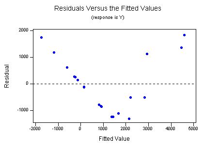
What does this
graph tell you concerning the validity of the Linear Regression Model in this
case.
Answer 7) The original data is not linear.
You
may want to see if taking the log of Y and re-running the regression gives a
more random looking residual plot, in other words, the log of Y and X may be
linearly related.