Intro
to Probability and Statistics
Sample
Final #1 – Questions And Answers (Answer Key)
Professor Brian Shydlo
Instructions:
1) Please
write your name: _____________________________________
2) There
are 10 questions totaling 100 points. Please be careful to answer all
questions. Partial credit will be given.
Question 1)
8 Points (Correlation and Covariance)
Question 2)
15 Points (Expected Value and Standard
Deviation of a Portfolio of Two Assets)
Question 3)
6 Points (Basic Probability and Binomial Distribution)
Question 4)
10 Points (Linear Regression, theoretical concepts)
Question 5)
23 Points (Linear Regression)
Question 6)
9 Points (Multiple Linear Regression)
Question 7)
8 Points (Testing Two Sample Means)
Question 8)
6 Points (Hypothesis Testing)
Question 9)
5 Points (ANOVA Comparison Of Means)
Question
10) 10 Points (Sample Means and Confidence Intervals)
Total
100 Points
Question
1) (8 points in Total)
You have
the following table of X and Y values.
(For example, there is a 10% chance that X will be 4 and Y will be 2,
and so on…)
|
X |
Y |
Probability(X,Y) |
|
4 |
2 |
10% |
|
6 |
4 |
20% |
|
7 |
7 |
20% |
|
10 |
14 |
20% |
|
12 |
15 |
30% |
To help you
out I have calculated the Standard Deviation and Mean (or Expected Value) of
each.
μx
= 8.6
μy
= 9.7
sx
= 2.8
sy
= 5.1
Question
1a) (5 Points)
What is
Covariance(X,Y)?
Answer: ___________________________
Answer 1a)
Covariance = 13.98
|
X |
Y |
Prob(y,x) |
X- μx |
Y - μy |
Prob(y,x) * (X- μx)
* (Y - μy) |
|
4 |
2 |
10% |
-4.6 |
-7.7 |
3.542 |
|
6 |
4 |
20% |
-2.6 |
-5.7 |
2.964 |
|
7 |
7 |
20% |
-1.6 |
-2.7 |
0.864 |
|
10 |
14 |
20% |
1.4 |
4.3 |
1.204 |
|
12 |
15 |
30% |
3.4 |
5.3 |
5.406 |
|
|
|
|
|
|
|
|
|
|
|
|
|
Sum = 13.98 |
Question
1b) (3 Points)
What is the
Correlation Coefficient of X,Y?
Answer: ___________________________
Answer 1b)
Correlation(X,Y)
= Covariance(X,Y) / (sx * sy)
so
Correlation(X,Y) = 13.98 / (2.8 * 5.1)
= 0.978991597
Question
2) (15 points in total)
A certain
stock, X, has an expected return of 15% per year and a standard deviation of
25%. The Stock is Normally Distributed.
A certain
bond, Y, has an expected return of 5% per year and a standard deviation of
9%. The Bond is Normally Distributed.
They have a
correlation of -0.2.
You could
write this as:
mx
= 15%, my
= 5%, sx
= 25%, sy
= 9%, and rxy
= -0.2.
Question
2a) (3 Points)
You decide
to invest $100 dollars in either X or Y or some combination of both. How do you allocate your $100 to maximize
your expected return?
Answer: ___________________________
Answer 2a) Invest all $100 in X.
Question
2b) (3 Points)
You decide
to split your money and invest $50 in X and $50 in Y. How much money do you expect to have after
one year (your initial investment of $100 + the expected return of your
portfolio of X and Y). (The correct
answer is some number over $100… I am not asking how much more money you would
have.)
Answer: ___________________________
Answer 2b)
$100
* (1 + [ 50% * 15% + 50% * 5%]) =
$100
* (1 + [ 7.5% + 2.5%]) =
$100
* (1 + 10%) =
$110.00
Question
2c) (5 Points)
What is the
standard deviation and variance of the portfolio from part b?
Answer: ___________________________
Answer 2c)
Variance(whole portfolio) = (Psx)2 + ((1-P)sy)2 + 2 * (Psx) * ((1-P)sy)) * rxy
Variance(whole portfolio) = (.5 * 25)2
+ (.5 * 9)2 + 2 * (.5 * 25) *
(.5 * 9)) * -0.2
Variance(whole portfolio) = (12.5)2 +
(4.5)2 + 2 * (12.5) * (4.5) *
-0.2
Variance(whole portfolio) = 156.25 + 20.25 + -22.5
Variance(whole portfolio) = 154
Standard Deviation of Whole Portfolio = sqrt(154)
= 12.41%
You get 3 points for getting something close.
Question
2d) (4 Points)
What is a
95% (1.96 standard deviation) confidence interval for your return? That is, give me a confidence interval for
50% in X and 50% in Y.
Answer: ___________________________
Answer 2d)
P[10.0
- (1.96 * 12.41) < μ < 10.0 + (2 * 12.41)] = 95%
P[10.0
- 24.32 < μ < 10.0 + 24.32] = 95%
P[-14.32
< μ < 34.32] = 95%
If
put
P[-85.68
< μ < 134.32] = 95% then OK
If
put
P[-83.25
< μ < 136.75] = 95% then -1 point
If
put
P[109.757
< μ < 110.243] = 95% then -1 point
Question
3 (6 points in Total)
Question
3a) (3 Points)
You have a
deck of card with 52 cards. It is a
standard bridge deck, which means it has 4 suits (hearts, clubs, spades and
diamonds). For each suit you have 13
cards: Numbered cards from 2 to 10, a Jack, Queen, King and an Ace.
Question
(3a): You pick 20 out of the 52 cards at random. What are the odds you'll see the Ace of
Spades?
Answer:
_____________________________________________
Answer 3a)
20/52
= 38.46%
This
could also be modeled as a hypergeometric distribution with x=1, n=20, M=1, and
N=52 (see the answer to the next question for details).
Question
3b) (3 Points)
With the
deck above you number each card from 1 to 52 so that the Ace of Spades gets a
Number of 1 and so on down to the lowest card, which gets a number of 52. Furthermore, you designate 26 (50%) of the
cards to be in the top half and 26 to be in the bottom half.
You observe
that for the 20 cards you picked out (one or a few at a time from the desk), 5
of them are in the top half and 15 of them are from the bottom half (in terms
of the ranking). Assuming that
everything is totally random, you decide to calculate the odds of getting 5 OR
FEWER cards in the top half when you draw 20 cards randomly from the deck as
described above.
You decide
to model this as a Binomial Distribution with a p, probability of success at
50% (since half of the cards are in the top half and half in the bottom
half). The formula you come up with is:
Sum from x
= 0 to 5 this: ![]()
Where p =
.5 and n = 20
Using this
formula (six times and taking the sum), you get a probability of 2.07% or about
1 in 50.
Question
(3b): Was your analysis/modeling of the problem above correct? If not, what is the problem with it?
Answer:
_____________________________________________
Answer 3b)
The
problem with the modeling above is that the binomial distribution assumes all
trials are independent. However, in the
above case, there is sampling without replacement. The correct formula is shown below:
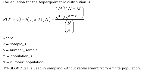
Where
you sum the result of x going from 0 to 5, n = 20, M = 26, and N = 52.
You
get an answer of 0.47%, or about 1 in 211.
This is less than ¼ the probability as with the binomial example. This is the correct analysis.
To
further illustrate the differences, if you were to take 40 cards from 52, there
would be zero percent change of getting 27 cards in the top half of the desk
(there are only 26 to begin with).
However, if you were to take one card at a time from the deck and then
put it back for 40 times, there would be a 1.09% chance of getting 27 cards in
the top half.
You
get 1 point for putting something down.
Question
4) (10 points in Total)
Question
4a) (5 Points)
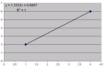
You have
this data (exactly two datapoints)
|
X |
Y |
|
1 |
2 |
|
4 |
6 |
You decide
to run a regression and you get an R-squared of 100%. Here is a chart:
Question
(4a): Why is it a bad idea to do a regression and especially make predictions
and especially create confidence intervals around those predictions when you
only have two datapoints?
Answer:
_____________________________________________
Answer 4a)
Here
I am looking for some reasonable answer.
Here is one possibility:
1)
With two datapoints, you'll always get a straight line right through the
points.
2)
You'll therefore always get an R-squared of 100%, which means the standard
error of the regression would be zero, which means that any confidence interval
would also be zero.
3)
Basically 2 points would never be enough to disprove the null hypothesis that there
is no relation between X and Y, yet the regression will always show a 100%
relationship.
You
get 2 points for putting something down.
Question
4b) (5 Points)
The Random
Walk theory of the Stock Market says that you can't predict what will happen with
the stock market. You tried to disprove
this, but so far no success.
One of the
models you used was to take the log of monthly returns for the S&P 500 from
Jan 1990 to April 2003 and then shift it by one month. You ran a regression of the shifted returns
(as the X) versus the unshifted returns (as the Y) and found there was no
relation. The R-squared was zero.
You decide
it is pointless to try to predict future market direction based on historic
data, so you decide to try to predict market volatility based on historic
volatility. You set up a model where
you calculate volatility using the previous 12 months. So you calculate the February 1991 volatility
of the stock market as the standard deviation of the log of the stock market
returns from February 1990 to January 1991 (12 Months). You calculate the March 1991 volatility of
the stock market as the standard deviation of the log of the stock market
returns from March 1990 to February 1991 (12 Months). And so on.
As before
you decide to shift the volatility by one month and try to predict the next
month's volatility based on the previous months.
This is an
excerpt of the Raw Data:
|
Month |
Montly_Volatility
(Y) |
Montly_Volatility_Previous_Month's
(X) |
|
Feb-91 |
4.986% |
5.294% |
|
Mar-91 |
5.294% |
5.289% |
|
Apr-91 |
5.289% |
5.179% |
|
May-91 |
5.179% |
4.675% |
|
Jun-91 |
4.675% |
4.931% |
|
Jul-91 |
4.931% |
5.059% |
|
ect… |
ect… |
ect… |
Here is
graph of the Data:
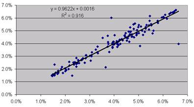
Here is the
Minitab output of the Data:
The regression equation is
Montly_Volatility = 0.00183
+ 0.952 Montly_Volatility_t-1
Predictor Coef StDev T P
Constant 0.001825
0.001016 1.80 0.074
Montly_V 0.95201 0.02410 39.50
0.000
S = 0.004233 R-Sq = 91.6%
Analysis of Variance
Source DF SS MS F P
Regression 1
0.027958 0.027958 1560.14
0.000
Residual Error 143
0.002563 0.000018
Total 144 0.030520
Question
(4b): At first you are thrilled with the 91.6% R-squared. Then you realize that a R-squared that high
is to be expected… meaning that the result is trivial.
In other
words, everything about your regression was totally accurate from a technical
point of view… low p-score, linear relationship, ect…, but the high R-squared
is a trivial result. Why?
Answer:
_____________________________________________
Answer 4b)
Here
I am looking for some response that indicates you are aware that the X and the
Y share 11 out of 12 source points that were used in calculating volatility and
therefore you would expect them to be similar.
Here
is one example of a correct answer:
When
you calculated the volatility you used 12 months of data. The volatility that was shifted 12 months
contains 11 of the 12 datapoints from the unshifted volatility (and one
different one). So you would expect the
Y to be 11/12 (11/12 = 91.6%) of the X since it contains 11/12 of the
data.
This
was pretty tricky.
Question
5 (23 points in Total)
You do a
regression of X against Y. You get these
results:
Regression Analysis
The regression equation is
Y = 12.2 + 0.533 X
Predictor Coef StDev T P
Constant 12.176 4.002 3.04
0.005
X 0.5334 0.1372 AAAA
0.001
S = 10.65 R-Sq = BBBB
Analysis of Variance
Source DF SS MS F P
Regression 1 DDDD CCCC
15.11 0.001
Residual Error EEEE
3288.7 113.4
Total 30 5002.2
Question
5a) (3 Points)
Predict Y
when X = 20
Answer:
_____________________________________________
Answer 5a)
Y
= 12.2 + 0.533 * 20 = 12.2 + 10.66 = 22.86
Question
5b) (3 Points)
Create a
95% Confidence Interval for your prediction.
Assume that 2.04 is the correct number for the t-distribution such that
95% of the data is between -2.04 +2.04 for the appropriate number of degrees of
freedom (in other words, use 2.04 when building your confidence interval).
Answer:
_____________________________________________
Answer 5b)
P
[22.86 - 2.04 * 10.65 < y < 22.86
+ 2.04 * 10.65 ] = 95%
P
[22.86 - 21.726 < y < 22.86 + 21.726] = 95%
P [1.134 < y < 44.586] = 95%
-2 Points for dividing by Square Root of N
Question
5c) (5 Points)
List 3
possible reasons why your confidence interval may be off or inappropriate.
Answer:
_____________________________________________
Answer 5c)
Accepted
responses (you just needed 3):
1)
The original distribution may not have been linear.
2)
The variances of the errors about the mean may not have been uniform, so your
confidence interval may be too wide or two small.
3)
The errors about the mean may not be normally distributed as assumed in the
regression model.
4)
An X of 20 may be outside the range of the original data, such that you may be
extrapolating and therefore your prediction may be suspect.
5)
You may have made a math error. (This
one is a stretch and not really what I was looking for, but I'll accept it).
Question
5d) (5 Points)
Fill in the
missing values from the Regression Output Table (1 point each).
AAAA:
_____________________________________________
BBBB:
_____________________________________________
CCCC:
_____________________________________________
DDDD:
_____________________________________________
EEEE:
_____________________________________________
Answer 5d)
AAAA
= 0.5334 / 0.1372 = 3.89
BBBB
= 1 - (3288.7 / 5002.2) = 34.3%
CCCC
= 113.4 * 15.11 = 1713.5
DDDD
= 5005.2 - 3288.7 = 1713.5
EEEE
= 30 - 1 = 29
Question
5e) (4 Points)
You do
another (unrelated) regression of a new X against a new Y. You have 10 datapoints. You get an R-squared of 80%, an F-score of 32
and a Standard Error of the Regression of 4.68188.
What is the
Standard Deviation of the variable Y?
Hint:
Make an ANOVA table based on the above information.
Answer:
_____________________________________________
Answer 5e)
S = 4.68188 R-Sq = 80.0%
Analysis of
Variance
Source DF SS MS F
Regression 1
701.44 701.44 32
Residual
Error 8 175.36 21.92
Total 9 876.80 97.4222
Step
1) Calculate the Degrees of Freedom
Step
2) Calculate MSE = (Standard Error of Regression)2
MSE
= 4.681882 = 21.92
Step
3) Calculate SSE
SSE
= MSE * DFE = 21.92 * 8 = 175.36
Step
4) Calculate SST
SST
= SSE / (100-80%) = SSE /20% = 175.36 / 20% = 876.80
Step
5) Calculate MST (which is also the variance of Y)
MST
= SST / DFT = 876.80 / 9 = 97.4222
Step
6) Calculate the Standard Deviation of Y
Standard
Deviation = Sqrt(Variance) = Sqrt(97.4222) = 9.87
You get 2 points for writing out an accurate ANOVA table.
You get 1 point for writing something looking like an ANOVA table.
Question
5f) (3 Points)
Your friend
does another (unrelated) regression of a new X against a new Y. Your friend get a low p-score of .00001 and
an R-squared of 4.6%. Everything else
with the regression checks out as being valid.
Your friend
decides to not use the Linear Regression model since it has such a low
R-squared. What do you tell your
friend about your friend's decision to reject the Linear Regression model due
to the low R-squared?
Answer:
_____________________________________________
Answer 5f)
Basically
I am looking something that indicates a low R-squared (so long as everything else checks out) is
still better than nothing, which is the percentage of variability that is
explained if you just use the average of the Ys to predict future Ys. I'll also accept something where you tell
your friend to try a Multiple Linear Regression model instead.
Question
6 (9 points in Total)
You get
some data regarding a batter. This is
it:
|
Hits |
Misses |
Total at Bats |
|
6 |
14 |
20 |
|
7 |
14 |
21 |
|
8 |
15 |
23 |
|
7 |
17 |
24 |
|
8 |
13 |
21 |
|
7 |
16 |
23 |
|
6 |
18 |
24 |
|
7 |
15 |
22 |
|
6 |
17 |
23 |
|
7 |
17 |
24 |
You decide
to run a Multiple Linear Regression to use Hits and Misses to predict Total at
Bats.
Question
6a) (4 Points)
What is the
Regression Equation (2 points of credit) and R-squared (2 points of credit)?
Answer:
_____________________________________________
Answer 6a)
Regression Equation Total at Bats = 1 * Hits + 1 * Misses
R-Squared = 100%
You
get 2 points for putting just the formulas down.
Question
6b) (5 Points)
You do
another (totally unrelated) Multiple Linear Regression. You have two variables, X1 and X2, which you
use to predict a third variable called Y.
This is the
output from Minitab:
Regression Analysis
The regression equation is
Y = 10.2 + 0.0605 X1 + 0.757
X2
Predictor Coef StDev T P
Constant 10.166 2.147 4.74
0.002
X1 0.06050 0.05639 1.07
0.319
X2 0.7569 0.1380 5.48
0.001
S = 0.6742 R-Sq = 82.8% R-Sq(adj) = 77.9%
Analysis of Variance
Source DF SS MS F P
Regression 2
15.3183 7.6591 16.85
0.002
Residual Error 7
3.1817 0.4545
Total 9 18.5000
Question (6b): Comment on the table
above, specifically commenting on the appropriateness of the Multiple Linear
Regression Model based solely on the above table of data. If the model is not appropriate in this
case, what might you do to make it better?
Answer:
_____________________________________________
Answer 6b)
The
p score for X1 is too high. Based on the
high p-score, try running the Regression as a Simple Linear Regression of X2
versus Y.
Question
7 (8 points in Total)
Question
7a) (5 Points)
An
interesting article was published recently that talked about why many of us are
feeling that things are getting more expensive even though the Consumer Price
Index is only 3%.
The article
describes the CPI (Consumer Price Index) as a basket of commonly purchased
items (e.g., Computer, TV, Mortgage, Clothing, furniture, cars, ect...). It goes on to say how items relating to the
maintenance of purchases (and one's self) are not included in the CPI (e.g.,
Health Care, Cable TV, Gasoline, Tuition, Car Insurance, Home Heating Oil,
Train Fare, ect…) are going up at a higher rate.
Below is
data meant to illustrate the kind of data from the article:
|
|
Consumer Price
Index |
Cost of Maintaining
Items |
|
Item 1 |
1.60% |
4.30% |
|
Item 2 |
2.40% |
4.60% |
|
Item 3 |
4% |
5.20% |
|
Item 4 |
2.80% |
6.90% |
|
Item 5 |
3.00% |
7.30% |
|
Item 6 |
1.00% |
8.90% |
|
Item 7 |
-4% |
|
|
Item 8 |
10% |
|
|
Item 9 |
6% |
|
You realize
that the average of the Non-CPI items is higher, yet you also realize that
there is a chance that all of these items may come from the same
population. You decide to run a T-test
for comparing two sample means. Here is
what you get:
|
t-Test:
Two-Sample Assuming Unequal Variances |
|
|
|
|
Consumer Price
Index |
Cost of Maintaining
Items |
|
Mean |
2.98% |
6.2% |
|
Variance |
0.001429444 |
0.0003232 |
|
Observations |
9 |
6 |
|
Hypothesized
Mean Difference |
0 |
|
|
df |
12 |
|
|
t
Stat |
-2.209418802 |
|
|
P(T<=t)
one-tail |
0.023664899 |
|
It is true
that the means are not equal? Please
formally state your conclusion and give reasons why.
Answer:
_____________________________________________
Answer 7a)
I'll
accept any valid answer. Since I didn't give
an alpha, I'll accept that you used an alpha of 5% or 1% (or possibly other
values).
For
an Alpha of 5% you would reject the null hypothesis. Why?
P-score is 2.3, which is less than 5%.
For
an Alpha of 1% you would accept the null hypothesis. Why? P-score is 2.3, which is more than 1%.
Question
7b) (3 Points)
Assuming
Unequal Variances is the more conservative approach: True or False?
Answer:
_____________________________________________
Answer 7b)
The
Answer is TRUE.
Question
8 (6 points in Total)
Write the
null and alternate hypothesis for the following items. This can be an English description or using
symbols.
Question
8a) (3 Points)
The ANOVA
test for comparing means:
Answer:
_____________________________________________
Answer 8a)
Null
Hypothesis: All means are equal
Alternate
Hypothesis: At lease one mean is not equal to the others.
Question
8b) (3 Points)
Multiple
Linear Regression:
Answer:
_____________________________________________
Answer 8b)
Null
Hypothesis: All slopes are zero
Alternate
Hypothesis: At lease one slope is not zero
Question
9 (5 points in Total)
Imagine you
run a customer service desk for a product with 5 customers. You record the number of Service Requests
each month and have these averages for year-to-date 2003:
|
Customer A |
Customer B |
Customer C |
Customer D |
Customer E |
|
14 |
9.4 |
8.8 |
16.2 |
10.6 |
The raw
data is:
|
|
Customer A |
Customer B |
Customer C |
Customer D |
Customer E |
|
Jan |
13 |
16 |
7 |
27 |
13 |
|
Feb |
10 |
11 |
5 |
21 |
6 |
|
Mar |
20 |
9 |
7 |
23 |
16 |
|
April |
18 |
5 |
18 |
7 |
14 |
|
May |
9 |
6 |
7 |
3 |
4 |
You run an
ANOVA test to try to determine if the means could really be the same. You get these results:
Analysis of Variance
Source DF
SS MS F
P
Factor 4
202.0 50.5 1.21
0.338
Error 20
836.0 41.8
Total 24
1038.0
Individual
95% CIs For Mean
Based on
Pooled StDev
Level N
Mean StDev ------+---------+---------+---------+
Customer 5
14.000 4.848 (---------*---------)
Customer 5
9.400 4.393 (---------*---------)
Customer 5
8.800 5.215 (---------*---------)
Customer 5
16.200 10.545 (---------*---------)
Customer 5
10.600 5.273 (---------*---------)
------+---------+---------+---------+
Pooled StDev = 6.465 6.0
12.0 18.0 24.0
What does
the test say about the possibility that all the means are equal?
Answer:
_____________________________________________
Answer 9)
Based
on the output, you can't reject at a reasonable level of significance the idea
that all means are equal.
Question
10 (10 points in Total)
You conduct
a sample of 64 items. Your sample mean
is 20 and you get a sample standard deviation of 10.
Question
10a) (3 Points)
Write out
the formula you would have used to calculate the Sample Standard Deviation?
Answer:
_____________________________________________
Answer 10a)
Square
Root [ Sum (xi - sample mean) / n-1]
Question
10b) (2 Points)
What is your
point estimate for the true population mean?
Answer:
_____________________________________________
Answer 10a)
20. The Sample Mean is your best estimate of the
population mean.
Question
10c) (5 Points)
Write out a
95% Confidence Interval for the True Population Mean. Assume that +-1.96 standard deviations hold
95% of the data.
Answer:
_____________________________________________
Answer 10c)
The
Standard Error of the Mean is 10/ sqrt(64) = 10 / 8 = 1.25
The
Confidence Interval is:
P[20
- 1.96 * 1.15 < mean < 20 + 1.96 * 1.15] = 95%
P[20
- 2.45 < mean < 20 + 2.45] = 95%
P[17.55
< mean < 22.45] = 95%
If
thought 20 was Standard Error (instead of Sample Mean) then got credit.
Extra
Credit 1 (1 Point)
The
Standard Normal Distribution has a mean of 0, a Variance and Std Dev of 1
The
T-Distribution has a mean of zero. Could
it have a Standard Deviation of Sqrt(df / df+2)?
Sqrt =
Square Root
df =
Degrees of Freedom
Don't just
give a True/False, explain why.
Answer:
_____________________________________________
Answer Extra Credit 1)
No. The Standard Deviation of the T Distribution
must be above 1. If df = 10, then the
equation would give a result of Sqrt(10/12) = 0.913.
For
the curious, the actual formula of the Standard Deviation of the T Distribution
is Sqrt(df / df-2).
Extra
Credit 2 (1 Point)
Half of the
numbers (meaning area under the curve) in a Chi-Squared Distribution are above
the Expected Value of the distribution.
Don't just give
a True/False, give a reason.
Answer:
_____________________________________________
Answer Extra Credit 2)
False. Half of the numbers are above the
median. The Expected Value is the
mean. These are the same if the
distribution is symmetric. Since the
Chi-Squared distribution is not symmetric (it is skewed to the right) then the
mean is not equal to the median. More
than half of the area is above the mean in this distribution.